Jupyter Notebook
When you are writing Python code for Tethys apps, you will most likely be working in an IDE such as PyCharm. To run code in your IDE, you will launch a browser and refresh your app in the Tethys virtual environment. There is nothing wrong with writing code this way, but it does involve a fair amount of overhead. For cases where you are just experimenting with code as you learn Python, you may want to use something simpler. Or in other cases, you just want a simple sandbox to get your code working before you attempt to deploy it in a Tethys app. For both of these cases, we encourage you to use Jupyter Notebooks.
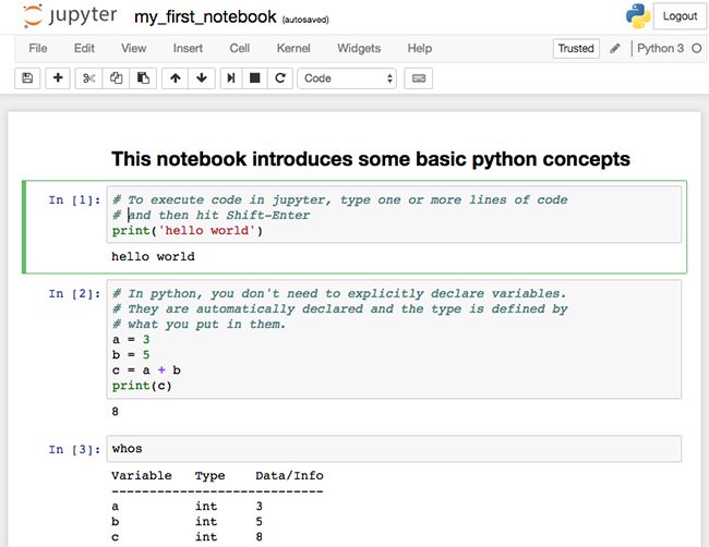
Jupyter is a free and open source application that runs in a web browser. You enter lines of Python code in blocks called "cells". Each cell can contain a single line of code, or several lines of code. You can execute the code in a cell by putting the cursor in the cell and hitting Shift-Enter. The output from that cell (if any) is then displayed directly below the cell. This allows you to incrementally develop your code and preserve the code and the output in a notebook file. It is particularly helpful to use the matplotlib graphics library with Jupyter. Here is some sample jupyter output:
Installing Jupyter
Before launching Jupyter, you need to make sure it is installed. If you followed all of the instructions in the Conda unit, you should already have it installed. You can check by opening a terminal and pathing to your home environment. They type:
$ conda list
Check to see if Jupyter is included in the list. If not, type the following:
$ conda install jupyter
and follow the prompts.
Launching Jupyter
Before launching Jupyter, you might want to create a directory to host your Jupyter files. Go to your home directory and type:
$ mkdir sandbox
then
$ cd sandbox
To launch Jupyter, type:
$ jupyter notebook
Now you should see a new window launch in your default broswer. The Jupyter home page shows you the contents of your working directory. The working directory is the directory where you launched Jupyter. If your code generates any files as output, it goes to the working directory by default. If you have any files or notebooks in the working directory, they would be listed like this:

Notebooks have the extension "*.ipynb". You can open a notebook in a new browser tab by double-clicking it.
Note: If you are using Chrome and Mac OS, you might get an error message and no new tab in the browser. This is a bug in either the OS or jupyter. You can get to the notebook by copying and pasting the URL shown in the terminal to a browser. You will then see the jupyter environment. To fix this problem, do the following:
Generate jupyter config if you don't have it:
$ jupyter notebook --generate-config
After executing this line, you will see a path to the config file. Use a text editor to open that config file and find this line:
#c.NotebookApp.browser = ‘’
and change it to:
c.NotebookApp.browser = u'chrome'
Be sure to take out the # comment sign. Save and try again.
My First Notebook
Let's create a new notebook and experiment with Python and Jupyter. We will start with some sample code that will teach us some basics about Python and how Jupyter works. Before starting, click on the following link to open in a new browser tab, or right-click on the link to download and open in a text editor.
This file contains the Python code associated with the exercise we wish to complete. We will copy and paste the code one cell as a time. Each cell is marked with the cell number as follows:
# In[1]:
Ok, let's begin:
1. Create a new notebook by selecting the New button on the right and then selecting Python 3.
2. Give it a name. Click on untitled at the top-left rename it to: “my_first_notebook”. This will create a new notebook in your working directory. Click Save icon periodically to save your changes as you go along.
3. You should see an empty cell. Copy-paste the first block of code, including the comment line.
# To execute code in jupyter, type one or more lines of code and then hit Shift-Enter
print('hello world')
Or you can type it manually. After entering the code, hit Shift-Enter. As you go along, remember that Enter creates a new empty line for Python code in the cells and Shift-Enter executes the code in the cell.
4. Copy-paste and run the next block of code:
# In python, you don't need to explicitly declare variables. They are automatically declared and the type is defined by what you put in them.
a = 3
b = 5
c = a + b
print(c)
5. One of the features of Jupyter is that you can go back to a previous cell and change the code and re-execute the cell. For example, go back to the first cell and change it to something like this:
# To execute code in jupyter, type one or more lines of code and then hit Shift-Enter
print('HELLO WORLD!')
and then select Shift-Enter.
6. You may wish to look through the Jupyter menus and shortcuts and experiment with them. Note that you can delete cells, insert new cells, and split existing cells.
Now that you have the basics down, continue all the way through the notebook code. Copy-paste the code for each cells and execute. Feel free to experiment. If you wish to see the solution, you can download it by right-clicking on the following link and downloading it to your sandbox directory:
You may need to refresh the Jupyter home page to have it show up. You can go through the sample notebook by putting your cursor in the top cell and then repeatedly selecting Shift-Enter.
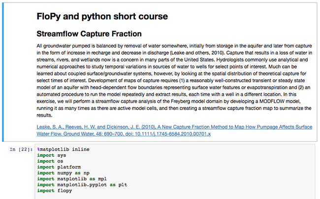
Advanced Notebooks
We have prepared some more advanced notebooks that will teach you how to use Jupyter notebook to solve tasks more typical of what you would put in a Tethys app. For each of these notebooks, right-click to download to your sandbox directory and then refresh your Jupyter homepage. Double-click on the notebook to open and use Shift-Enter to go through each cell and view the output.
| Notebook | Description |
|---|---|
| nwm_example_basics.ipynb | This notebook uses a REST API to query the National Water Model at a specific reach identified by a COMID for a specific forecast to download a time series of the predicted hydrograph for the reach. The hydrograph is plotted with matplotlib. |
| nwm_example_waterml.ipynb nwm.20170604.zip nwm.20170613.zip |
This notebook does the same thing, but uses a Python library specfically designed for the WaterML format. It also includes code to print gridded output from the NWM. For this notebook to work properly, you will also need to download and unzip the two zip archives shown on the left in your sandbox directory (or whatever directory you are using to lauch jupyter). |
| ecmwf_sfp_examples.ipynb | This notebook uses a REST API to query output from the ECMWF Streamflow Prediction Tool. You pass in a date and stream reach ID to return a current forecast. |
| grace_example.ipynb | This notebook uses a REST API to query a Tethys app hosted at BYU associated with the GRACE satelite data. It passes a lat/lon coordinate and the API returns a time series of change in total water storage (in cm depth) for the GRACE cell coincident with the selected point. |
As you go through the notebooks, you may get an error message on some of the import statements saying that the indicated library is missing. If so, just go to the command line and use Conda to install the missing package as follows:
$ conda install <missing package name>
And again, feel free to modify the code and experiment. That is what Jupyter notebook was designed for!
Markdown Cells
You can comment the code in your Jupyter notbooks using standard Python comments, but you can add comments and narrative that are much more readable using markdown cells. Markdown looks like this:
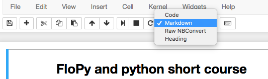
To create a markdown cells, make a new cell and then change the format from Code to Markdown using the the selector in the Jupyter menu.
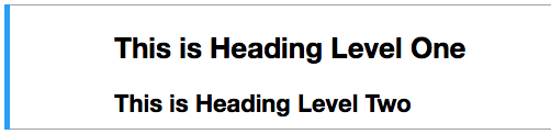
Markdown is a text formatting or markup language used by many websites, including GitHub, Reddit, Stack Exchange, and SourceForge. It uses simple markers in the text to convert raw text to formatted text. For example, to make headings you type:
# This is Heading Level One
## This is Heading Level Two
Then select Shift-Enter and you get:
Here are some links describing how to use Markdown:
https://github.com/adam-p/markdown-here/wiki/Markdown-Here-Cheatsheet
https://daringfireball.net/projects/markdown/syntax
Quitting Jupyter
As you use Jupyter, you will notice that a series of messages will be displayed in the terminal window where you launched Jupyter. When you are through with the exercises in this unit and you wish to quit Jupyter, you can either kill the terminal or go to the terminal window and type Ctrl-C.
IPython Command Line
If you ever need to quickly test some Python code, you may also want to try the IPython command line. This gives you access to the kernel used in Jupyter, but without the overhead of the web interface. Just go to the command line in the terminal and type:
$ IPython
You can then type your code one line as a time. For example:
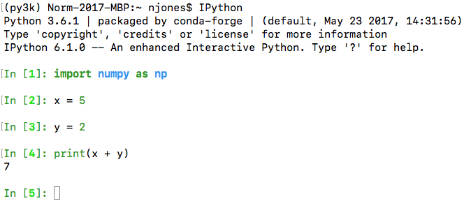
See www.ipython.org for more information.