Running Predictive Simulations

The completion of the groundwater model for the Goulbi Maradi aquifer opens up the possibility for predicting future scenarios by modifying the input data. This will provide valuable insight into potential changes in water resource availability, which is crucial for informed water management decisions. To achieve this, entry files will need to be altered to reflect different conditions or assumptions about the future, such as changes in the recharge, groundwater pumping rates, and other relevant factors. The outcome of these future scenarios will provide a basis for proactive measures to ensure sustainable water resource management.

To simplify this process, we have documented a set of steps that can be used to model the files and run the simulations. There is one section below for pumping rates, one for recharge, and one explaining how to process the results.

Changing the Pumping Rates

The first step in predicting future scenarios for the groundwater in the Goulbi Maradi aquifer is to adjust the pumping rates for the wells. The well is ulimately saved in the MODFLOW Well Package input file. However, we will use a feature in GMS that allows us to change the pumping data easily by importing a CSV (Comma-Separated Values) file describing a pumping schedule into GMS and GMS will then save the new pumping rates to the MODFLOW input files.The pumping rates for the model are recorded in 14 separate Excel files, each corresponding to a different zone in the model. Changes can be made to one zone at a time. The modified rates are then saved in CSV (Comma-Separated Values) format, and imported to GMS.

The pumping data files are stored in a set of Excel files in the Wells folder that is downloaded with the predictive model files.

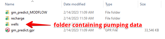
There are 14 wells files corresponding to the 14 pumping zones:

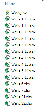
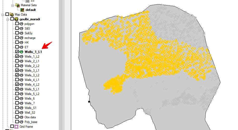
You can determine the spatial extent of each zone by loading the model in GMS and then selecting the well point coverages listed in the Map Module. You can also see a map of the well region in the Excel files as explained later in this document.

Each Excel file consists of 6 columns: ID (name), X and Y coordinates, pumping rate, date, and time. Each well has 4 rows that are associated with three important dates and associated pumping rates: 1) the date of construction, 2-3) the date range over which we have data for calibration, and 4) the date at the end of the simulation. Typically the last row is the only one that changes, as it is used to update the model to use a new future pumping rate.

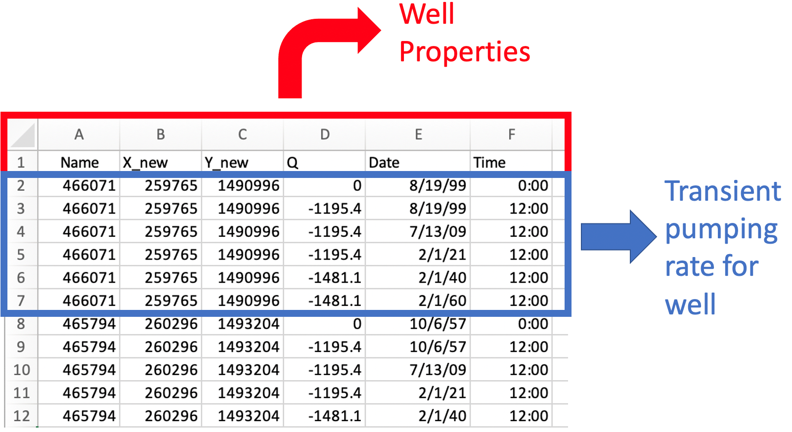
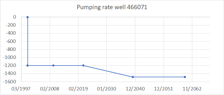
These dates and rates represent a time series indicating how the pumping rate changes over time. For example, The well named 466071 had an estimated pumping rate of -1195 cubic meters per day (m³/day) until February of 2021. The pumping rate predictive in this examples for this well in February 2060, ~40 years in the future, will be 1481.1 m³/day. This a linear increase in pumping over time, with the future rate being 1.24 times higher than the initial estimate. This rate is assumed to be representative for the region and is applied to all wells in the region.

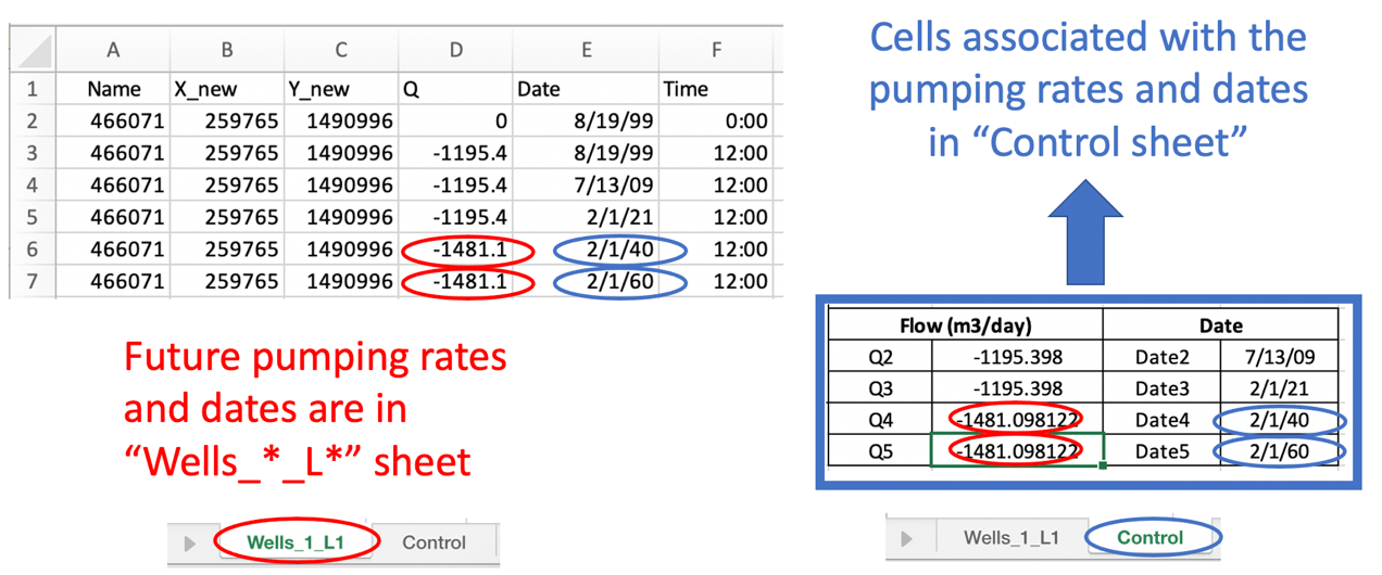
The pumping rate predictions for well ID 466071 are associated via a set of formulas with four cells in “control” sheet, named  Q2, Q3, Q4, Q5, Date2, Date3, Date 4 and Date5. By modifying the value in cell Q5 and Date5, the predictive pumping rate and the date can be easily updated and the changes will be automatically reflected in the pumping rates for all wells in the “Wells_*_L*” spreadsheet. This makes it convenient to adjust the predictions as needed. Typically, you would only change the Q5 value.

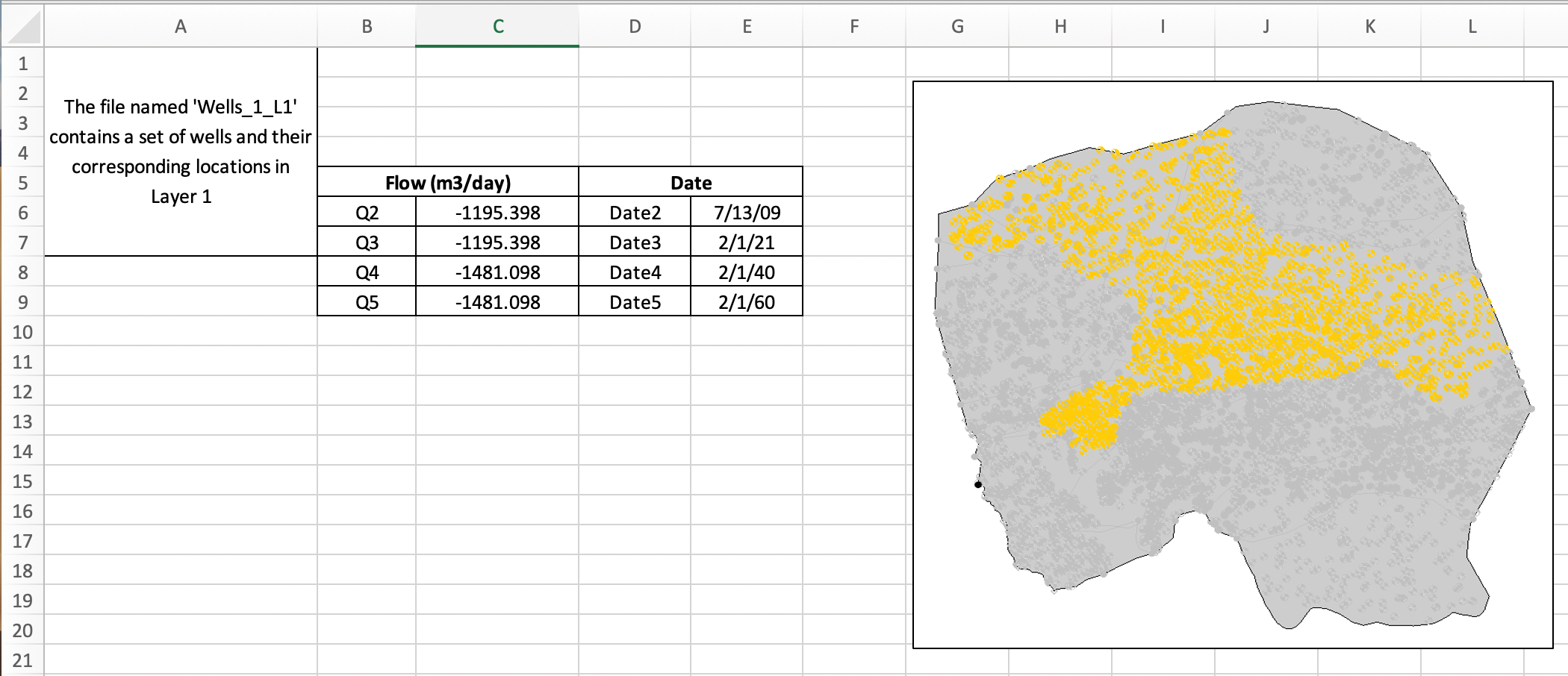
Additionally, it is possible to observe in the “control” spreadsheet, the number and the location of the well associated with each file.

To prepare a tabular pumping rate data file for import into GMS, you need to follow these steps:

1. Change the future pumping rates and dates as desired in the control spreadsheet.
2. Save the file with a *.csv extension to ensure it is in a format that can be easily imported into GMS and to export only the “Wells_*_L*” spreadsheet.
3. In GMS, select the coverage that corresponds to the name of the *.csv file and use the "File|Open" command to open the text import wizard.
4. In the text import wizard, turn on the heading row box

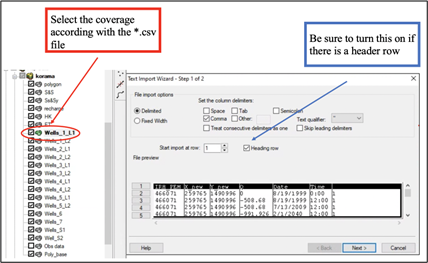
5. In the text import wizard, turn on the heading row box and click Next.
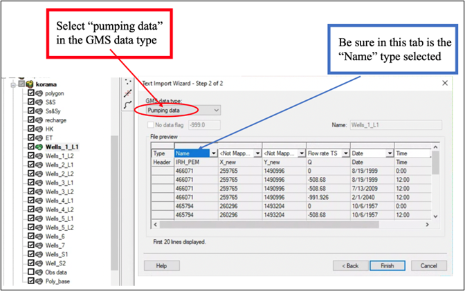
6. Select “pumping data” in the GMS type, be sure in the type tab is selected the option  “Name” as shown in the figure below and click finish.

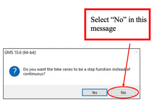
7. Finally, select option NO to the message shown in the figure below. This process will allow you to import the updated pumping rates into GMS and use them in your modeling work.

At this point, the pumping data have been updated for the selected region in the GMS conceptual model. To convert the conceptual model data to MODFLOW grid data:

8. Go to the Feature Objects menu and select the Map -> MODFLOW command. Click OK at the prompt.
9. Save the project to a new file name and run MODFLOW

This can be repeated for other zones you wish to change. You can change multiple zones before step 8 and then convert the zones and run MODFLOW once.

Also, you may wish to come up with other pumping strategies. For example, you could create a future pumping schedule corresponding to staged or step-wise set of changes in the pumping rate. To do this, you would simply need to modify the entries for each of the wells to add new rows corresponding to points on the pumping time series.

It should be noted that the predictive simulation starts in 2002. In theory, it could be set up to start in 2020. We calibrated the model using calibration data over the period 2002 - 2009. The pumping rates, recharge, etc from 2009-2020 were assumed, but were calibrated based on how the change in groundwater storage matched the storage changes observed in the GRACE-derived groundwater storage estimate. As part of running the predictive model, you may wish to modify these assumptions. However, if the model were changed to start in 2020, the future predictions would run much faster.

Modifying the Recharge Estimates

Groundwater recharge is important to consider in groundwater modeling because it is the main source of water to an aquifer and assumptions about recharge have a critical impact on the model results and determine how much water can be pumped from the aquifer. Recharge is sensitive to land use changes and irrigation practices, but it is primarily a function of recharge and it can be impacted by climate change.

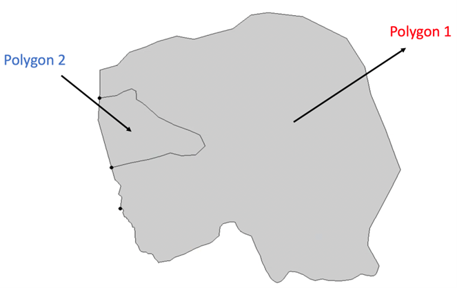
The Goulbi Maradi aquifer is characterized by a uniform land use and land cover, and the model has been set up with only two recharge polygons to control the groundwater recharge. This distribution of recharge made it possible to calibrate the model, but it should be changed for predictive simulations.

To modify the recharge estimates for the Goulbi Maradi aquifer, the excel file with the date and recharge values can be used. The file is located here in the download package:

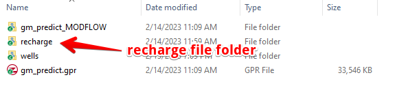
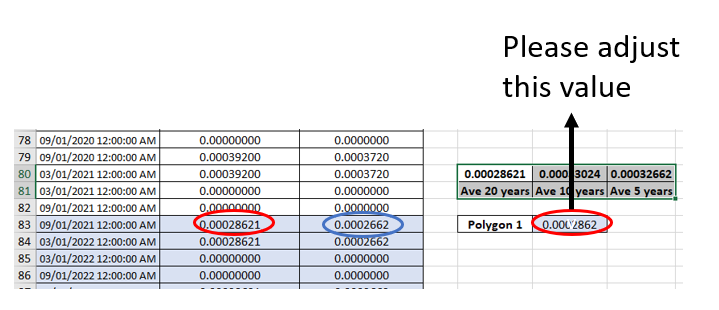
The file is called recharge_predictive.xlsx. This file provides a detailed description of the recharge rate, allowing for an accurate assessment of the groundwater resources in the area. In the Excel file, there are three columns associated with the date and the recharge estimates for polygons 1 and 2, respectively.

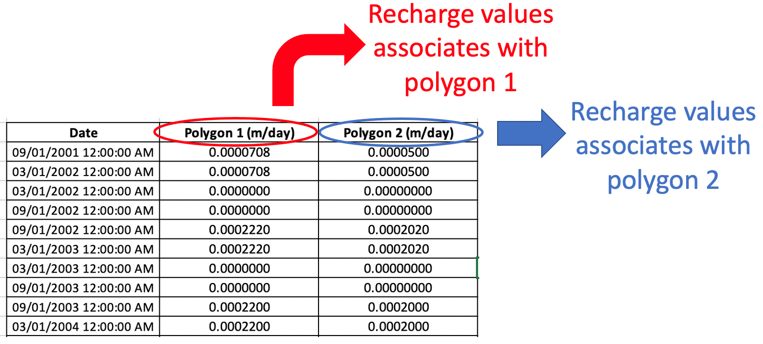
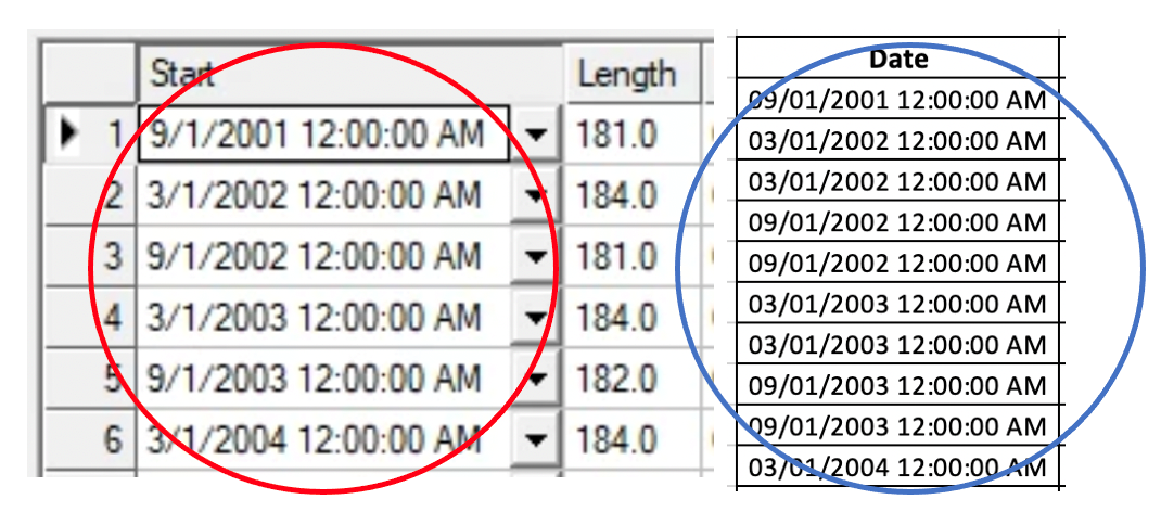
The start date is September 1^st, 2001, and the end date is March 1^st, 2060. These dates are linked to the stress periods, so it's crucial to maintain consistency. If you modify the dates, ensure to also update the corresponding dates in the stress periods.

fe

The figure presents the average annual groundwater recharge, depicted in blue, which was calculated using the two approximations of the Water Table Fluctuation method until February 2021. The two colors represent polygon 1 (blue) and polygon 2 (orange). Polygon 2 has a rate that is 0.00002 m/day less than Polygon 2. After February 2021, the blue and orange values represent the predicted future groundwater recharge, which represents a value around the average of the values from ~2017-2021. This assumption can be modified as described below.

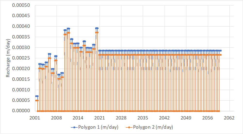
To modify the future groundwater recharge, represented by the blue cells from March 1^st, 2021 to March 1^st, 2060, proceed in a manner similar to what we did for the pumping rates case. Simply adjust the value in the cell labeled "Polygon 1" to apply a new constant recharge from 2021 to 2060, as shown below (make sure have the "Recharge" tab selected in Excel). Note that the recharge values for Polygon 2 are maintained at 0.0002 m/day less than the values for Polygon 1. If the recharge is not constant or if you wish to use a different pattern entirely, you will need to manually change the values in the table for each period or modify the formulas.

After making changes to the recharge in the Excel file, you need to update the data in the groundwater model. To do this, we will use a simple copy-paste approach as follows:

1. First select the recharge coverage, and then right-click and choose the "Attribute Table" option.
2. In the attribute table, select "Polygons" in the Feature option, and then click the three dots (as shown in the right figure below) associated with the polygon for which you want to change the recharge.

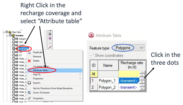
3. To access the recharge rates dialog, click on the three dots. As shown in the figure below, a window will open.
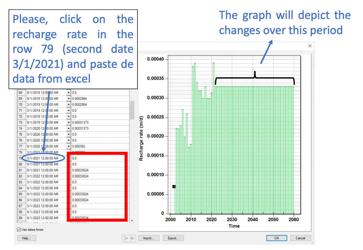
4. Then copy and paste the recharge rates column for Polygon 1 from Excel for the period after February 2021, which was estimated using the Water Table Fluctuation method, into the recharge rates dialog.
5. Repeat the previous steps for Polygon 2.

Note that the recharge rates after this period are predictions. Do not modify the recharge rates prior to March 2021 , as this may impact the model's calibration.

Finally,

6. Click OK to exit the dialogs.
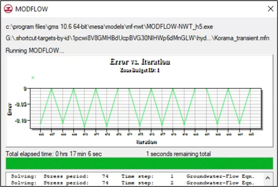
7. Right-click on the Recharge coverage and select the Map->MODFLOW command.
8. Save the project to a new filename and run MODFLOW.

The model is transient, and a 60-year simulation is being run, so the actual run time may be as long as 15 to 20 minutes depending on the computer.

Viewing and Processing the Results

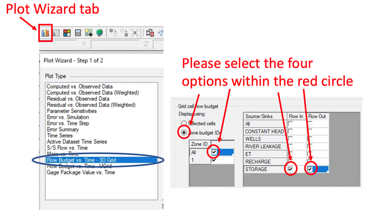
After reading the solution in GMS, you can step through the time steps and view the head contours and see how they change with time. You can also use the Plot Wizard option in GMS to calculte the changes to the flow budget and then copy the flow budget to a spreadsheet we have prepared to view plots showing how the flow budget has changed based on the modifications you made to the model. To do this, click on the "Flow Budget vs. Time - 3D Grid" option, then click "Next." The window displayed on the right will appear. In that window, please select the four options within the red circle.

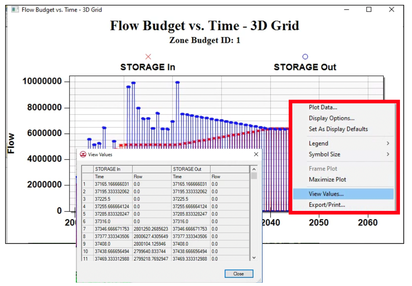
Click on the "Finish" tab and the graph for the selected options will appear. In the Plot Wizard, you can observe and modify the graph. However, for this exercise, please right-click on the figure and select the "View Values" option, and then copy the displayed data.

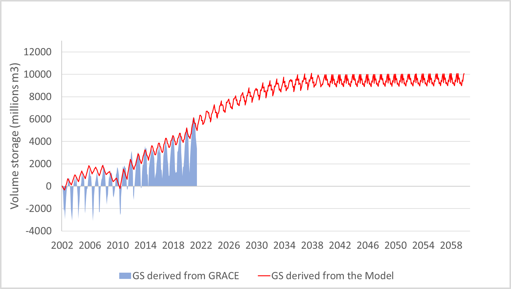
Please paste the data in the designated column of the "Transient Results" excel file. The information will automatically be updated and a comparison between the storage estimated using GRACE data and the storage computed with the model results will be displayed in the graphic.

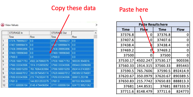
As an example, recharge is estimated using the average of the last 10 years and pumping rates are increased by 1.24 times. Under these conditions, the results indicate an increase in groundwater storage from 2022 to 2036. Beyond 2036, the storage level remains steady until 2060.